Clive’s Corner #9: Introducing a demonstration microscope.
Clive’s Corner by Clive Bagshaw
A feature of MicroNews, Clive’s Corner is a place created for the sharing of knowledge, tricks, and tools. The Corner is where you read about clever microscopical hacks - and submit your own. Clive’s Corner is the namesake of SFMS member Clive Bagshaw, who has spent a lifetime looking into microscopes - including 50 years studying protein reactions.
There is an unwritten rule for Clive’s Corner that do-it-yourself microscope modifications should cost $20 or less. Just as well it is unwritten because this hack will cost about $50 – but then you get a complete working microscope with Köhler illumination for this. The purpose is to construct a demonstration microscope with accessible optics so that the light path can be followed all the way from the lamp to the eyepiece. If you are puzzled by real and virtual images, finite and infinite optics, conjugate focal planes and magnification factors or want to teach others about these aspects, then this tool is for you.
First, a trip to the local hardware store to obtain a 24 inch (600 mm) steel shelf rail (not aluminum) and a pack of grip clips to hold 1 inch (25 mm) diameter components (you will need 5 or 6 clips in total ). You will also need some nuts, bolts and 6 mm diameter magnets to attach the clips to the rail. These components will form our optical bench. Next, four 1 inch diameter magnifying glasses will provide the optics. A cheap set of four loupes are available on-line. These are labelled 5x, 10x, 15x and 20x although these magnifications are overestimated by 2- to 3- fold (see below). Thirdly a flashlight, with a single LED chip and an adjustable front focusing lens is required as a light source. Finally, an iris diaphragm is useful to demonstrate the field and condenser apertures. These components are shown in Figure 1.

Figure 1a. Grip clip with two 6mm magnets attached.

Figure 1b. Set of magnifying loupes.

Figure 1c. Components required for the demonstration microscope. From top left: “10x” eyepiece, card screen for primary image display, “20x” objective lens, sample slide, “15x” condenser lens, “5x” supplementary collector lens, adjustable iris diaphragm and LED flashlight with focusable collector lens. Below: optical rail with grip clips in approximate position before fine adjustments.
First, we will make an optical bench. To allow for repositioning of the lenses, stick two magnets to the base of each grip clip with a dab of superglue, close to the hole but no further apart than the width of the rail, as shown in Figure 1a. Once the final position on the rail is established, the clip can be secured with a nut and bolt, although some clips will need the freedom to slide for fine adjustment. You may need to drill out the slot in the rail, depending on the size bolt you use. You will need to stick magnets on all the clips so that the center height of each component is the same.

Figure 2a. Business card in binder clip with magnet on the base.
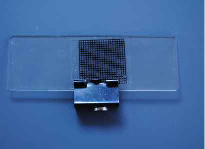
Figure 2b. Test slide with a 1 mm grid mounted in binder clip with magnet on the base.
Let us make a simple microscope (i.e., a magnifying glass) by attaching a clip to the lefthand end of the rail. This clip can be fixed with a bolt as it will be a constant in all the arrangements we explore. Place the nominal “10x” loupe in the clip, with the lens itself on the lefthand side. For an object, use a white business card, held in a small binder clip to which a magnet has been glued the base (Figure 2a). Position the card on the rail and move it until the writing on the card is in focus when viewed through the lens. Measure the distance from the card to the lens within the loupe – it should be around 75 mm. This is the focal length, f, of the lens. The image we see is described as virtual, rather than a real image because it does not appear on a screen but rather just on our retina via the eye lens. The focal length of the eyepiece lens can also be determined by projecting a real image of the sun onto the card - the sharpest image is formed 75 mm from the lens. The magnification power is defined relative to what we see with the unaided eye when viewed at the closest distance for comfortable viewing. This distance is usually taken at 250 mm (around 10 inches) which is a rather ageist standard. The magnification is then defined as M = 250/f = 250/75 = 3.3x for the “10x” loupe. When the eye is positioned close to the loupe, the magnification becomes M = (250/f)+1 = 4.3 x. Either way, these values are significantly less than the label attached to the loupe (Table 1).

Table 1. Magnification of Loupe lenses when used a magnifying lens or microscope eyepiece. The numerical aperture defines the efficiency of light collection, NA = n Sin α, where n = refractive index of the medium (= 1 for air) and α is the half angle subtended by the lens when parallel light is brought to a focus e.g., for the “10x” loupe, Sin α = half diameter/focal length = (20/2)/75 = 0.13 and α = 7.7 degrees.
So much for a simple microscope. Now let’s make a compound microscope by attaching the “20x” loupe to the rail via a magnetic clip at about 180 mm from the “10x” loupe clip, with the lens itself pointing to the right. This is our objective lens with f = 30mm. Make a test object by drawing an X on a glass slide with a marker pen, or better, use a stick-on 1 mm grid. Mount the slide on the rail using a binder clip and magnet (Figure 2b). Place this about 40 mm from the “20x” lens and look through the “10x” eyepiece and move the slide until it comes into sharp focus. You may need to hold the rail towards a light or the sky (not the sun!) to get a bright enough image to see. Now attach the LED flashlight to the righthand end of the rail via a clip, magnet and bolt and replace the business card to its original position of 75mm from the eyepiece lens. Turn on the LED and you will see an image of the slide on the business card. Fine adjust the position of the slide to get the sharpest image. This is a real image, unlike the virtual image seen through the eyepiece. With the slide at 40 mm from the “20x” lens the image will be about 120 mm from the lens, in agreement with the thin lens formula 1/u + 1/v = 1/f, where u is the object distance and v is the image distance (i.e., 1/40 + 1/120 = 1/30). The real image magnification formula M = v/u = 120/40 = 3, shows the “20x” loupe is behaving as a 3x objective lens under these conditions. With a 1 mm grid as the test slide, the grid image will show gradations 3 mm apart. Magnifications are only meaningful when related to a particular pair of object and image distances and we are not following any particular standard microscope tube length at this point (more below). The position of the image seen on the card at 120 mm from the objective lens is called the primary (or intermediate) image plane. If the test slide is moved a few millimeters away from the objective lens (i.e., an increase in u), the image distance, v and the magnification decrease.

Figure 3. Primary image formation in a compound microscope with a finite tube length.

Figure 4. (a) Controlling the light intensity of the LED using a 10K ohm potentiometer (b) as a variable resistance. (c) The negative terminal of the battery holder is soldered to the black wire and the red wire is soldered to the connector to the switch. (d) In normal operations these terminals make contact but here an insulator is made from a piece of plastic, so the current goes through the resistance. Setting the potentiometer resistance to zero results is the normal brightness of the LED.
We can also view the primary image through the eyepiece with LED illumination. Before you do try this, you need to attenuate the LED flashlight so as not to be dazzled. This can be done by sticking a piece of white paper over the LED flashlight to reduce its intensity. A better method, for flashlights where the battery compartment is accessible, is to add a 10K ohm variable resistor in series with a battery terminal connector (Figure 4). This will enable continuous adjustment of the LED intensity. When viewed through the eyepiece, the total magnification of the compound scope is 3 x 3.3 = 10x for the combination of the “20x” objective and “10x” eyepiece (i.e., don’t believe the labels!)
Let’s take a closer look at the LED light source. You will note the LED flashlight has a squarish chip about 1 mm in size (Figure 5a - it will look bigger when viewed through the focusing lens). When shone on a wall about a meter away, the LED chip can be brought into focus by moving its lens forward and reveals the square chip about 40 mm across at 1 meter distance and some fine lines between the LED components. When used in our demonstration microscope, much of the light from the LED is wasted because it diverges to an area much bigger than the objective and the eyepiece lenses, even at minimum focus. We need to condense the light further using an additional lens(es). To get the brightest image, we could focus the LED chip onto the slide itself – this is termed critical (or source-focused) illumination, but it gives uneven lighting due to the fine structure within the LED chip. To see this effect, place the “15x” loupe about 55 mm to the right of the slide. The primary image will show the test slide illuminated by the bright square shape of the LED. When sharply focused by adjusting the position of the condenser lens and/or the LED focusing lens, the fine structure within the LED chip may be seen (you may need to reduce the LED intensity to see this effect). Defocusing the LED chip image away from this position reduces the problem of unevenness, but a better solution to get the most even illumination across the field-of-view is to use Köhler illumination. Here we use an additional light collection lens, the “5x” loupe, in front of the LED to bring the LED chip image in focus at the front focal plane of the “15x” condenser lens i.e., 55 mm to the right of the condenser lens (Figure 5b). This is achieved by placing the “5x” loupe about 120 mm to the left of the LED clip and by fine adjustment of the LED lens. Now the light emitted to the left of the condenser shows little convergence nor divergence as it passes through the test slide towards the “20x” objective lens (so-called infinity space). It is brought to focus at 30 mm to the left of the objective lens – the so-called back focal plane of the objective. Placing the business card at this point reveals a bright image of the LED chip, well separated from the primary image plane that is 120 mm to the left of the objective lens. Another way to even out the illumination of the sample, often used in cheaper microscopes, is to use a diffusion disk in front of the light source (Figure 5c). However, for more critical studies, such as phase contrast and differential interference contrast (DIC) it is best to have full control over the imaging and illumination foci, as in Köhler illumination.
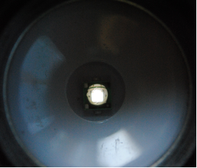
Figure 5a. The flashlight LED chip observed after removal of the focusing lens.

Figure 5b. Image of the LED chip at the front focal plane of the condenser when set up for Köhler illumination – note the fine grid like structure within the LED image.

Figure 5c. A diffusion plate made from a yogurt pot lid used as an alternative to minimize local structure in the LED chip at the sample plane.
The multiple positions where objects are brought into focus are term conjugate planes (Figure 6). Thus, the front focal plane of the condenser and the back focal plane of the objective lens are conjugate planes and are distinct from the sample plane, which is conjugate with the primary image plane and your retina when looking through the eyepiece (ATTENUATE THE LED BEFORE LOOKING HERE!). The sample plane is also conjugate with a plane to the right, close to the LED focusing lens. This can be seen by placing an iris at this point. On closing the iris, the leaves of the iris will be in focus with the primary image plane and restrict the field-of-view (Figure 7a,b). Hence, at this position, it is termed the field iris and is used to match the field-of-view of the objective/eyepiece combination. The precise position of the field iris can be determined in the demonstration microscope by temporarily placing the LED flashlight in the position of the “20x” objective lens and finding the image of the sample slide using the card. In effect the condenser and collecting lens constitute a microscope facing the opposite direction. Returning to the original layout, if the iris is placed at the front focal plane of the condenser, closing the iris reduces the angle of light reaching the objective lens and passed a certain point (when the numerical aperture of the condenser lens is less than that of the objective), it reduces the overall intensity of the light which illuminates the sample, but has a limited effect of the field-of-view (Figure 7c,d). Due to the relative long focal lengths and small numerical apertures of our loupe lenses (Table 1), the overall effects of the condenser iris on the angle of illumination are not well demonstrated here and are best observed on a real microscope with a higher numerical aperture condenser (see Clive’s Corner #1).

Figure 6. (a) Illumination conjugate planes where the LED chip is in focus. (b) Imaging conjugate planes where the test slide is brought into focus. The yellow beams represent the on-axis optical paths.

Figure 7. (a) and (b) the effect of closing the field iris reduces the diameter of the primary image. (c) and (d) the effect of closing the condenser iris is to reduce the intensity but leaves the field diameter unchanged. Note the primary purpose of the condenser iris is not to control intensity but the angle of illumination which effects the resolution and contrast of the image.
The loupe lens are single lenses (apart from the “20x” which is made up of 2 lenses) with limited optical quality and the grip clips are not precisely symmetrical, so the image suffers from aberrations and the light path will not be exactly centered. However, the demonstration is sufficient to illustrate the principles described above. It is possible to substitute the eyepiece and objective lens with real microscope components. When using a 160 mm tube length objective lens, you should mount the components such that the eyepiece shoulder, that rests on the eyepiece microscope tube, and the objective thread are 160 mm apart. When the test slide is at the optimal position, the primary image plane should be 10 mm to the right of the eyepiece shoulder and likely within the eyepiece barrel. Except for low power (≤ 4x) objectives, the back focal plane is likely to be within the objective barrel. This is why cheap loupe lenses are better than microscope lenses to demonstrate the basic principles. Note that the objective and eyepieces will still function at other separation distances (and give different magnifications) to give a reasonable image at the low resolutions we are exploring but aberrations are not corrected optimally.
The demonstration microscope can be used to model infinity-corrected objectives, but an additional tube lens is required. In this set up, the test slide is placed exactly one focal distance to the right of the objective (i.e., 30 mm for the “20x” loupe) so that the light leaving to the left of the objective lens remains parallel. A tube lens is required to focus the beam at the primary image plane. The advantage of this design is that additional components can be added within this “infinity space” (e.g., fluorescence filter cubes) without changing the aberration corrections required within the objective and eyepieces. A suitable set up uses the “5X” loupe as a tube lens, the “20x” loupe as the objective, the “15x” loupe as the condenser and the “10x” loupe as an additional collector lens placed close to the LED flashlight (Figure 8). The LED lens should be adjusted to bring the LED chip into focus at the front focal plane of the condenser, as before, to achieve Köhler illumination. The distance between the objective lens and tube lens is not critical as the imaging beam is parallel at the point (i.e., infinity space). The primary image plane will be exactly one focal distance to the left of the “5x” loupe (i.e., 110 mm). An additional eyepiece lens can be used to view the virtual image when positioned one focal length to the left of the primary image plane, but for demonstration purpose we can look at the real primary image on focused on the card. The conjugate planes of this set up are shown in Figure 9. Note that the yellow light beams shown in Figures 6 and 8 relate to the light path when exactly on the optical axis. For finite-sized objects, the off-axis light path will zig-zag through the lenses. For this reason, some divergence will be seen in the “infinity space” which limits the separation of the lenses to about twice the sum of their focal lengths rather than infinity. Beyond this distance the image will suffer from vignetting.

Figure 8. Demonstration of an infinity-corrected objective lens, using the “5x” loupe as a tube lens to produce the primary image on the card.

Figure 9. The conjugate planes of a microscope with an infinity objective lens. (a) the illumination path with Köhler optics (b) the imaging path with the test slide at the front focal plane of the objective.
The demonstration microscope can also be used to illustrate the basics of confocal microscopy (Figure 10a). Here we use a low power (<5 mW) laser slide pointer as a light source and remove the collector lens so that the laser enters the condenser as a parallel beam and is focused to a diffraction-limited spot on the test slide (i.e., critical illumination, Figure 10b). With a loupe lens the limitation more likely arises from the aberrations of the lens rather than the wavelength of light itself. Also, in a real confocal microscope the laser beam diameter is expanded to several millimeters to match the numerical aperture of the lens which minimizses the spot size. The objective (and tube lens in an infinity ‘scope) magnifies the spot, but it still remains a spot in the primary image plane (Figure 10c). DO NOT ATTEMPT TO LOOK THROUGH AN EYEPEICE when using a laser pointer. In a real confocal microscope, a pinhole is placed in the optical path at a conjugate position and a photon detector measures the intensity of light that passes through the hole. The pinhole removes out-of-focus light and reveals a very thin optical section of the sample.

Figure 10a. A non-scanning confocal microscope with a 5 mW laser.

Figure 10b. Focused laser beam on the test slide i.e., the small blue spot.

Figure 10c. Image of the laser beam at the primary image plane, one focal length from the tube lens.
Okay, a spot on its own may not be too impressive but to get an image we would need to scan the spot across the test slide. On commercial confocal microscopes this is done by moving the stage or using scanning mirrors to direct the beam. In our demonstration scope we can move the grid slide horizontally and see that the spot on the imaging card oscillates in intensity as a black grid bar coincides with the spot. In a scanning confocal scope, the intensity versus time record is converted into an image on the video monitor. Even a non-scanning confocal microscope has its uses. When the sample comprises a very dilute solution of fluorescent or light scattering particles, the spot will fluctuate in intensity as the particles enter and leave the laser beam by chance and the fluctuation frequency provides a measure of the diffusion constant of the particles. This was used to confirm the Stokes-Einstein equation proposed many years before confocal microscopy was a reality.
For further information about optics and microscopy Sanderson’s Understanding Light Microscopy is an excellent source.