Clive’s Corner #11: Magnification Problems Demagnified

One of the first things we learn about compound microscopes is that the total magnification of the system is obtained by multiplying the objective magnification by the eyepiece magnification e.g. a 40x objective lens with a 10x eyepiece gives an overall magnification of 400x. For our Victorian ancestors this information was fine, but these days it can lead to much confusion when labelling photographs captured through a microscope. The problem is that the above formula applies to the effective magnification as seen by eye. Here, the number refers to the magnification relative to that seen when looking at the same object with the unaided eye at 10 inches/25 cm distance ( see Clive’s Corner #9). As soon as you record the image on a camera, then additional factors apply, such as where the camera is positioned, whether the camera is used with or without additional lenses or an eyepiece, the physical size of the camera sensor, and the size of the video screen or page used to view the final image. Consequently, when publishing an image in a book or on-line, defining the magnification in the legend with the classical “objective times eyepiece” formula is next to useless. Rather, a scale bar should be added to the image at the time it is produced so that the true size of the object can be judged no matter what the size screen or page on which the image is eventually viewed.

Fortunately, the days of digital imaging have made adding a scale bar relatively straight forward – all you need is a standard calibration slide (also known as a stage micrometer or graticule; Figure 1). These graticules typically have calibration lines 10 µm apart, with a full scale of 2,000 µm (= 2mm) and can be used with both low- and high-power objectives. The principle is simple – take a digital picture of the graticule, calculate how many pixels correspond to a known length, use this number to draw a line of known length on the image of the subject taken with exactly the same microscope settings. In practice, this procedure is usually straightforward because a scale bar option is included in the software supplied with many basic of digital microscope cameras. If no such option exists, free software such as ImageJ can be used to apply a scale bar after capturing the image. Whatever procedure is used, the calibration procedure needs to be repeated for each objective lens and camera set-up. The calibration process can be saved for later recall although, for really critical studies, it is best to compare with the standard graticule each time because the camera magnification depends on the exact position of the camera - normally the camera is positioned to be parfocal with the eyepieces, but the latter depends on an individual’s eyesight.

a.

b.

Figure 1. (a) A slide graticule, (b) close-up of the central circle containing a 2 mm long scale

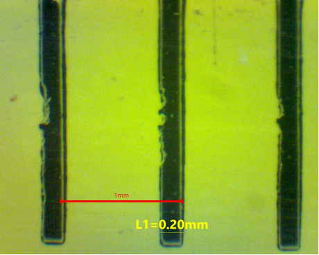
If you don’t have a calibration slide, then an ordinary ruler can be used at a pinch (Figure 2). Using the lowest available magnification, take a picture of the mm divisions (hopefully the field of view will span at least 1 mm – if not use a dissecting microscope). Once the number of pixels corresponding to 1 mm is determined, calculate the width of one of the lines on the scale (typically around 200 µm). Now go to the next highest magnification setting and use the width of the ruler line as a standard distance to apply a scale bar. This method can be repeated to cover the full set of objective lenses by choosing a small object in the field-of-view for the next higher power objective lens. The method is not as good as using a proper calibration slide because systematic errors maybe accumulated at each step – but it is better than nothing.

a.

b.

Figure 2. (a) Image of a mm ruler taken under a low-power stereo microscope. The scale bar was added using the spacing between the lines as 1 mm. The width of the line was determined using the “measure” option as 0.2 mm (200 µm). (b) End-on view of a USB eyepiece camera (outer diameter = 23.2 mm) showing a rectangular chip that is much smaller than the primary image as seen through an eyepiece lens.

Alternatively, if you know the size of the camera sensor and the number of pixels, you can calculate the expected magnification. For example, I have a 1.3 MP USB camera with a 3.6 mm wide sensor which is positioned at the primary image plane of a 160 mm tube length compound microscope (Figure 2b). The camera sensor comprises 1,280 x 1024 pixels. The standard 10X eyepiece has a field number of 18 mm. That means if I was to image a 1.8 mm long object with a 10x objective lens, the primary image would be 18 mm in length and would just fill the field when viewed by eye. However, the camera can only capture the central 3.6 mm of the primary image, so it would appear to give a further magnification of 18/3.6 = 5X compared with the view by eye. The actual magnification of the camera depends on the screen used for viewing the image. For example, if a 14 inch (~ 360 mm) monitor is used, the total magnification would be 360/3.6 = 100, times the initial magnification of the objective (10x), i.e. 1,000X overall compared with the 100X when viewed directly by eye with a 10X eyepiece. This camera, when used with a 10x objective lens would give an image where 1 pixel corresponds to 0.36 * 1,000/1,280 = 0.28 µm in width. These numbers depend on the accuracy of the specifications and the exact positioning of the camera at the primary image plane, so direct calibration with a graticule is preferable. However, the value of 0.28 µm per pixel is particularly interesting, as will be described in a future Corner.

One challenge with calibration arises when taking pictures through a microscope eyepiece using a camera with zoom capabilities. This applies to the usual procedure when using a smartphone. Here, zooming gives an additional magnification which requires photographing the slide graticule with exactly the same settings. The same problem applies to some stereo microscopes with zooming capabilities.

Aside from slide graticules, there are also eyepiece graticules which are useful for estimating sizes when viewing live images by eye. They are positioned at the primary image plane within the eyepiece. Eyepiece graticules need to be calibrated for each objective lens using a slide graticule on the stage. Once calibrated, they provide a solution to the problem of using a camera with zoom capabilities, as the graticule will be superposed on the image when photographed through the eyepiece. However, it does not help in the case of stereo microscopes with zoom adjustments of the objective lens setting.

Once a microscope/camera combination is calibrated using a slide graticule, a scale bar can be added to images of samples and/or the dimensions of specific objects can be determined. The exact process varies in different software, although the principles are the same. Below are summaries using 3 different programs.

Swift SwiftCam (Windows version)

1)     Select “Calibrate” under “Measure” menu (Figure 3a).
2)     Drag the scale bar to superimpose the graticule scale and extend it to overlay a known length in the horizontal direction.
3)     Click on x=y in the menu (this assumes the pixels are exactly square which is adequate for most purposes). The vertical scale will now match the horizontal scale.
4)     Enter the actual distance as measured by the graticule in the X-ruler unit and Y-ruler unit boxes (e.g. 100 µm in Figure 3b).
5)     Click on the SaveTo box and name the file with the objective magnification (e.g. 10x obj scale)
6)     Once saved, the Ruler_Setting box can be closed by clicking on OK.
7)     Repeat the above procedure for each objective lens.
8)     Switch to the sample of interest and open the “Calibrate” window as in step 1).
9)     Click on the LoadFrom and open the appropriate calibration file for the objective in use.
10)  Select “Line” under the “Measure” menu.
11)  Draw a line across the object of interest. This will show the actual length of the object (Figure 3c).
12)  To save the calibration on the image, go to “SaveOption” under the “Option” menu and tick “Measure” and/or “Ruler” boxes (Figure 3d).

For a video of the above procedures, click this link.

Figure 3. Calibration procedure using SwiftCam in Windows

Amscope (Windows version)

1)     Select “Calibrate” under “Options” menu. 
2)     Adjust the red line to span a known distance across the graticule.
3)     Enter the Magnification of the objective (e.g. 10x) and the actual distance (e.g. 100 µm, Figure 4a) and click OK.
4)     Then select “Scale Bar…” under “Measurements” menu (Figure 4b).
5)     Define the length of the required scale bar and click OK.
6)     To save the scale bar on the image Select “Merge to Image” under the “Layer” menu.
7)     To measure the length of a specific object, go to “Line” under “Measurements”, then select appropriate line (e.g. horizontal, Figure 4c) and draw a line the length of an object. Click at the end of the line and a number should appear which represents the length.
8)     To save the calibrated line on the image Select “Merge to Image” under the “Layer” menu.
9)     The name of the magnification selected in line 3 (e.g. 10x objective), should appear as an option in a dropdown toolbar which can be selected for later images, along with another option to change the units (e.g. mm or µm).
10)  Repeat the calibration procedure with different objective lenses.

Figure 4. Calibration procedure using Amscope software in Windows

ImageJ (free software)

This program can be used to add a scale bar to existing images provided a calibration graticule photographed under the same conditions is available. The software is useful for many forms of image processing and analysis. A browser version of ImageJ is also available. To add a scale bar:

1)     Draw a line to span a known distance on the graticule image.
2)     Select “Set Scale” under the “Analyze” menu (Figure 5a).
3)     Enter the line length in the “Known Distance” box and add the appropriate “Unit of Length” (Figure 5b).
4)     Tick the “Global” box so that this calibration is applied to subsequent images.
5)     Load an image of the sample obtained under the same microscope settings.
6)     To add a scale bar, select “Scale Bar” under the Analyze/Tools menu (Figure 5c)
7)     To measure a specific distance, draw a line over the object, then select Measure under the Analyze menu. The distance will be given in the Results window (Figure 5d). If the image is uncalibrated, the Length will default to the number of pixels.

See link for more details.

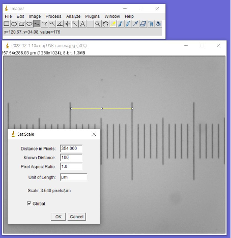
Figure 5. Adding a scale bar and measuring lengths using ImageJ software