Clive’s Corner #14: Pushing the Limits
The function of a microscope is to enable us to see objects that are too small to resolve with the unaided eye. This begs the question, how small an object can we see with a microscope? It turns out this is not quite as simple a question as it first might seem. There is a difference between resolving an object from neighboring things and detecting an object against its background. The resolution limit of a light microscope is of the order of the a few hundred nanometers (just under a micrometer, µm) and depends on the wavelength of light (λ) and the numerical aperture (NA) of the objective lens. That is, objects in the field of view must be separated by a distance of at least d in order to be distinguished.
d = λ/2*NA
Table 1 provides the values of d for a range of commonly used objective lenses with 500 nm (green) light, assuming no other aberrations contribute to the image.
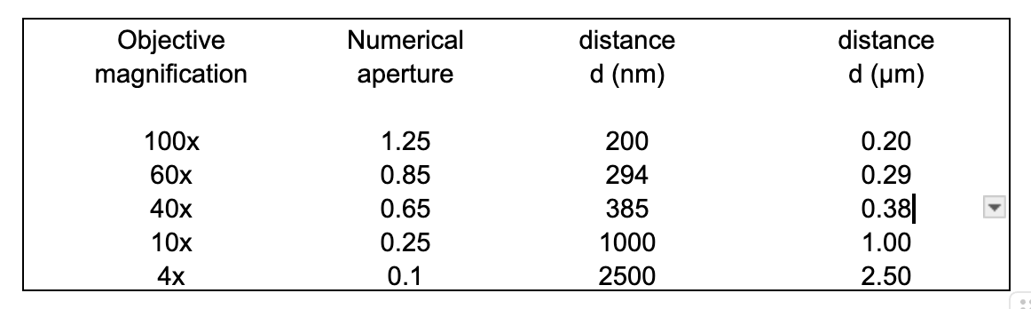
Table 1
Any object whose size is less than d, may still be detectable provided the signal is strong enough to distinguish it from the background. However, the object will appear blurred with an apparent size of the order of d, even if its physical size is much smaller.
Research-grade microscopes are often checked for performance by imaging 50 to 100 nm diameter polystyrene beads. The blurred image of the bead defines the Point Spread Function of the objective lens. This information can be used to computationally sharpen images and gives a gain in resolution of about two-fold (i.e. d is reduced by 2). If the microscope is correctly aligned, a cross section through the blurred image will show an intensity that follows a gaussian (bell-shaped) profile. This property is taken to the extreme in single molecule microscopy. Here, single fluorescent molecules with a size of 0.5 to 1 nm are imaged to give a blurred spot with a diameter of several hundred nanometers. This is possible in very dilute solution, where the average separation distance between molecules is > 10 µm so that the spots rarely overlap. The challenge here is to detect the weak fluorescence against the background. This requires a number of technical tricks, of which reducing the volume of the sample illuminated is key. Confocal and total internal reflection fluorescence microscopy are common means to achieve this.
At this point you might be wondering why anyone would be interested in looking at a very blurred image of a single molecule. On a personal note, it was the rekindling of my interest in microscopy. I had not looked through a microscope for 20 years since school biology classes and had focused on protein biochemistry as a research career. Electron microscopy was the only way to see protein-sized objects, but this was limited to static samples in a vacuum. When single-molecule light microscopy became possible, individual molecules labelled with different color fluorophores could be watched combining, reacting and separating in real time – a chemist’s dream. Figure 1a shows an image of individual Alexa 647 dye molecules obtained using a total internal refection fluorescence microscope and excitation with a HeNe laser at 633 nm. The image was obtained by summing the intensity over 10 seconds during which time most of the fluorophores bleached. Usually this occurred as a one-step process, confirming a single fluorophore was involved, but occasionally two-step photobleaching was seen due to overlapping unresolved molecules. The intensity variation reflects the time before a particular molecule bleached. Bright spots represent molecules which, by chance, survived longer in the laser beam and emitted more fluorescent photons. When an individual spot is enlarged, it can be seen that the image is spread over several pixels of the camera (Figure 1b). However, with good signal to noise, the center of the spot can be calculated to a precision down to 30 nm (Figure 2). This procedure provides the basis of one way to achieve super-resolution with a light microscope; STORM (stochastic optical reconstruction microscopy). Some dyes, such as Alexa, show reversible photobleaching and can be reactivated by shining light of a different color (488 nm blue light in the case of Alexa 647). First, an organelle within a cell is labeled with a photoactivatable fluorophore at a concentration such that the fluorophores overlap and give a blurred image limited by the d value as in conventional fluorescence microscopy. Then most of the molecules are bleached to an extent that the remaining molecules are well separated in space and their individual locations are calculated with nanometer precision. Following total bleaching, a few molecules are reactivated by illumination with a second color and the center of each fluorescence spot is calculated. Over time, different molecules are activated and analyzed so that the underlying structure of the organelle is built up with a higher resolution.

a.

b.

c.
Figure 1. Fluorescence from single Alexa647 molecules. (a) A field of single molecules imaged and averaged over 10 seconds. (b) An individual molecule averaged over 10 seconds. The expected resolution for the emitted 700 nm (far red) light with a 1.2 NA lens is 290 nm. (c) An individual molecule averaged over 0.1 seconds, limited by random photon arrival times. In (b) and (c) the pixel width is equivalent to 130 nm after magnification by the objective and tube lenses.

a.

b.

c.
Figure 2. (a) An individual Alexa647 molecule as in Figure 1b. (b) A Gaussian fit to average out pixelation. (c) Contrast enhancement and thresholding to locate the most likely position of the molecule (peak of the Gaussian fit) to within a precision of about 30 nm. Scale bar for all panels = 500 nm.
The images in Figure 1 were obtained 20 years ago with a Zeiss Axiovert microscope, a 63x 1.2 NA C-apochromat water immersion lens and an Andor electron-multiplying CCD camera (totaling around $60,000), not to mention lasers, high blocking fluorescence filters and associated optics. This is hardly the stuff of Clive’s Corner. But it does raise the question – what can be seen with a $200 Amscope microscope and a $10 laser pointer. As a test object, I used a zero-mode waveguide (ZMW) chip – a discarded consumable from a Pacific Biosciences DNA sequencer. A ZMW chip comprises a surface containing a grid of 150,000 nanowells with dimensions 70 nm diameter and 100 nm deep, separated by 10 µm. When samples are added at low concentrations, these wells may contain just a single fluorophore and the evanescent field from the side walls of the nanowell gives an enhanced fluorescence signal, allowing sensitive monitoring of single-molecule reactions. As a test of resolution of the Amscope microscope, the ZMW chip was mounted on the stage and illuminated with a green laser (532 nm) pointer mounted at about 45° to the stage as described previously (Clive’s Corner #13, Figure 2b). Light scattered by the nanowells was readily detected and produced spots that were about 1.4 µm diameter when using a 10x, 0.25 NA Amscope objective lens (Figure 3). Compare this with the theoretical 1.06 µm diffraction-limited value expected for this wavelength (cf. Table 1). In this case it is likely that spherical aberration of the objective lens contributes to the blur.

a.

b.
Figure 3. Light scattering from 70 nm zero mode waveguide (ZMW) wells imaged with an Amscope 120 microscope using a 10x 0.25 NA objective, a 1.3 MP USB camera and illuminated with a green (532 nm ) laser pointer. (a) Field of nano wells, separated by 10 µm. (b) Enlargement of 4 wells showing image is spread over about 5 pixels, each of which corresponds 0.28 µm in object space, i.e. overall spot diameter = 1.4 µm.
Apart from a resolution test, this result highlights another characteristic that has to be considered by practically all microscopists – how many pixels does a camera require to record photomicrographs and avoid pixelation being a limitation? This question depends on the size of the camera chip, its location in the microscope and any magnifying or reducing lenses in the optical path. The image of Figure 3 was obtained using a 1.3 MP Amscope eyepiece camera located at the primary image plane with a 10x lens. This camera has a sensor size of 3.6 x 2.8 mm with 1290 x 1024. The physical size of a pixel situated at the image plane is therefore 2.8 µm which means, after 10x magnification, it is equivalent to 0.28 µm in object space (Clive’s Corner #11). It can be seen that the ZMW image diameter is about 5 pixels, showing the pixel size is sufficiently small as not to be limiting. While it might seem prudent to have more pixels just to be on the safe side, there are disadvantages of using a camera with pixels much smaller than the diffraction-limit. Reading out a pixel is accompanied by a small background noise, so one larger pixel gives a better overall signal-to-noise ratio. Also transferring the data from the camera chip takes longer with more pixels, slowing down the maximum frame rate for videos. Indeed, the $30,000 camera used to record single Alexa647 molecules in Figure 1 had just a 0.26 MP chip (512 x 512) as the most important characteristic here was low read-out noise and high sensitivity to monitor single photons. Magnification with accessory lenses was arranged such that the final image covered just a few pixels which was a compromise between positional accuracy and signal intensity.
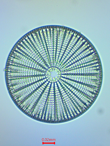
Single-molecule imaging may represent cutting-edge science, but it has little aesthetic appeal and is not easily accessible to the amateur. Early microscopists used the fine features of diatoms for resolution testing which are available to anyone with a net and access to pond or seawater. Figure 4 shows Arachnoidiscus ehrenbergii images obtained with different numerical aperture Amscope objectives. In (b) – (d) the images are enlarged to approximately the same scale and show that with reduced numerical aperture, the image becomes more blurred. Figure 4e shows a further enlarged section, obtained at NA = 0.1, to demonstrate that the pixel size is comparable to the blur due to lens aberrations and diffraction limited resolution.
a.

Figure 4. Resolution comparison of an Arachnoidiscus diatom using different objective lenses. (a) Overall image obtained with a 10 x 0.25 NA Amscope objective lens. (b) Image obtained with 60x 0.85 NA objective lens. (c) Enlarged section obtained with 10x 0.25 NA objective lens. (d) Enlarged image obtained with a 4x 0.1 NA objective lens. (e) Enlarged section from (d) showing smoothed image (top) and raw pixelated image (bottom). All images were obtained with 1.3 MP USB eyepiece camera at the primary image plane.
Using a camera with more pixels would give no advantage, resolution-wise, in this set up. Nevertheless, a camera with more pixels AND a larger sensor size would give an advantage of capturing a larger field-of-view. The 1.3 MP eyepiece camera only images the central 1/5 of the diameter seen through 10x eyepieces with a field number of 18. Apart from using a camera with a larger sensor, an additional lens may be positioned in the imaging path to project a magnified or reduced image size to match the sensor size. This comes with its own advantages and disadvantages …. and provides opportunities for more “Corners”.